This is my amateur dive into Spiking Neural Networks.
First up let me preface this by saying I am not a machine learning (ML) expert, nor software engineer. I am a mechanical engineer with an interest in ML who dabbles in code. In this case, I have intentionally avoided formal curricula to leave room for "creative misinterpretation". My ideas are half baked and perhaps somewhat misguided, my code is scrappy, but it does mildly interesting things. Please feel free to email me at blog@spec.nz if you'd like to reach out.
This is all about SNN's (Spiking neural networks). The world is obsessed with transformer models. There doesn't seem to be anywhere near as much interest or material out there on spike based networks. In terms of capabilities, today, SNN's are well behind other models. But I don't think we should give up on them. They have something that todays todays SOTA models overlook... Time.
SNN's are fascinating to me because of their parallels with the brain and the simplicity of the Hebbian learning and spike timing dependent plasticity (STDP) learning rules. My gut feeling tells me the so called 'path to more general intelligence' could involve some combination of state space models, recurrent neural networks and... spikes.
I figured experimenting with SNN's is a good way to gauge their potential. Others have built tools, but I've always wanted to build my own toy model from scratch. Something interactive to see what is happening under the hood, and to share it with others.
This is what I've created after a few months of tinkering. Is it revolutionary? No. Am I reinventing the wheel? Probably, who cares... Enjoy.
In theory, SNN's can learn patterns (coincidences). In particular, spatiotemporal patterns which is great for speech/audio and vision systems. What's more, they encode information in spikes (event based) rather than the more common ANN's that process data at fixed intervals. This has some unique advantages.
My approach?
I am going to attempt to strip away all of the complexity of regular SNN's to the point where all that is left is binary weights and simple addition and subtraction operators. I don't think it is necessary to simulate every millisecond of neuronal activity using exponential equations to calculate action potentials and model complex dynamics between all neurons at once. This is computationally heavy. I want to limit calculations to nodes that are actually firing and to encourage sparsity in the weights so we don't waste computing clock cycles on idle neurons. My thinking is if I can lower the computational requirements enough, then perhaps I can get something interesting happening, even in JavaScript!
Simplified LIF SNN Model
LIF = Leaky integrate and fire. An action potential regime for a simple neuronal model that integrates (accumulates) stimulus signals (inputs), fires/spikes when above a threshold, and leaks over time to a resting value.
Network Input Data Overview
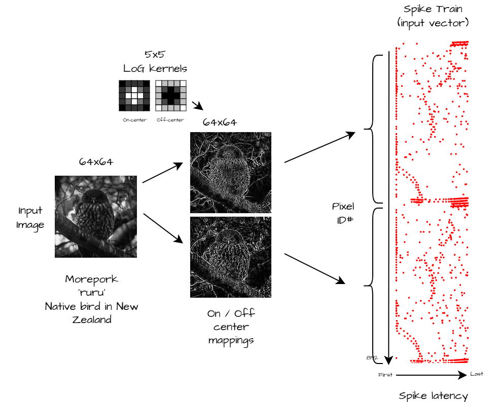
We start with an input image. Convert it to grayscale and down sample to 64 x 64px. Then we use a pair of 5x5 Mexican hat convolutional filters to produce on-center and off-center contrast maps. We do this because you often don't need entire 8-bit grayscale values for every pixel in an image to tell what the image is, just the edges can be enough, and this takes a lot less processing when you reduce it to this level. In this case the filters emphasize regions with high luminosity gradients (aka edges) while suppressing uniform regions. Though, if you wanted to perform other types of processing you easily could, e.g. raw pixel values, only the brightest spots, orientation maps, the differences between camera frames, or all of these at once. In fact you could use any combination of data making this "multi-modal", but you'd still want to select appropriate preprocessing/filters for the data type (e.g. spectrogram for sound, letters or tokens for text).
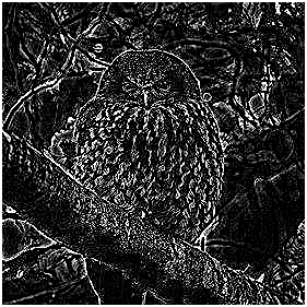
Next, with the resultant maps we convert/encode them to a "spike train". To do this we take every pixel ID and put it into one of 256 bins based on intensity. The bins are fed into the network in descending order such that the high intensity pixels have the lowest latency (fire first). These high intensity/low latency bins contain the most salient information about the image, and thus the first output node to fire as a result of the input spike train will likely also be the most important. For most images you can discard a lot of the lower bins (i.e. pixels with low contrast) and you will still recognize the image. See sample below. Though if you are trying to detect a dimly lit object in the shadows of an otherwise very bright image this approach will not work as we are throwing away that information.
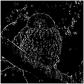
Contrast map of size 281x281 (78,961 total pixels)Same image but we apply a threshold so only the first bin is shown. In this case we have reduced it to only 4,559 pixels (spikes) (only 6% of the original)Animation where we alter the number of spikes (bins) included in the spike train. Notice how the image is still recognizable even using just the using minimum number of spikes.
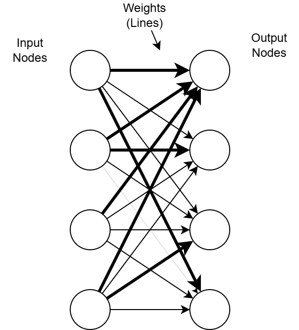
You may be used to seeing neural networks drawn with circles and lines like below. This makes it easy to see the network structure but not so easy to visualise the weights.
Single layer neural network drawn the traditional way
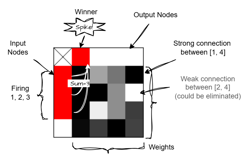
For a fully connected single layer network it can be drawn in a grid like fashion as below. This allows you to see the individual weights easier. Note: as a simplification this layer only shows 4 input nodes and 4 outputs and 16 weights. To process a 64x64px image we would need an input size of 8192 (2x 64x64 maps) and the number of outputs can be as few or as many as we want. The idea is that each output node will become receptive to a single pattern. The more outputs available the more capacity the network has to 'learn'.
Equivalent diagram drawn as a gate array
Inside the network, we fully connect each input node (left most column on diagram above) to every output node (top row) with a weight (shown on the main grid). The weights are initialised randomly to low values. The shade of each cell in the grid indicates the strength of the connection ranging from 0-1.
When an input node fires, it only stimulates its connected nodes according to the connection weights. The spikes accumulate in the output nodes and if any node is pushed above its threshold it fires. In a multilayered network this would then stimulate nodes in the next layer.
After each time step all nodes will slowly decay (leak) to their resting value. That is the essence of a spiking neural network!
Learning Rules
The network described above won't do much on its own. We need some additional mechanisms to get it to learn patterns. To recap what we are trying to achieve:
To automatically learn repeating patterns/coincidences/motifs
Promote connection sparsity. This is the key to reducing the memory and compute requirements
Prevent multiple nodes learning the same thing
STDP (simplified)
In terms of computing, this simplified learning rule is fast to calculate because it only requires addition and subtraction operations.
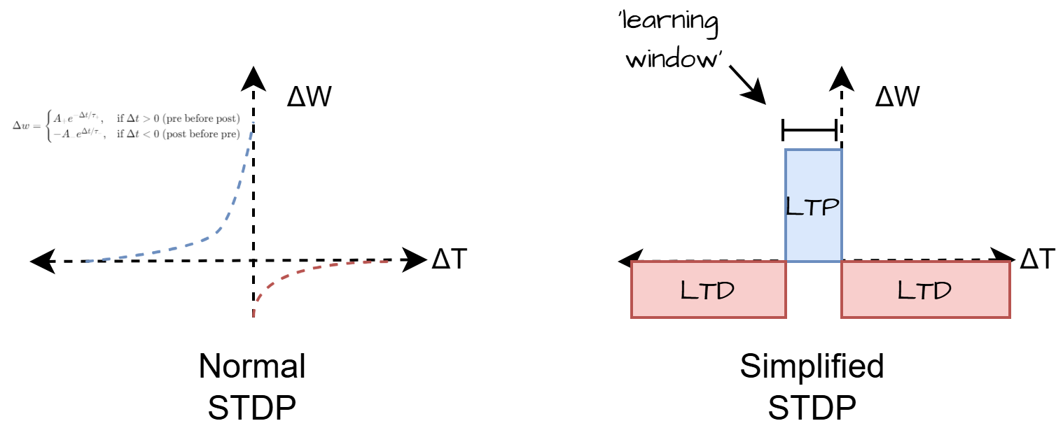
The core learning method here is STDP. Usually STDP is performed using an exponential function to precisely calculate the weight change based on relative timing between spikes. Here we reduce this function to something more binary. When a node fires there is a fixed weight increase (LTP - long term potentiation) if the pre-node fired within a fixed 'learning window', and then everything else is decreased (LTD - long term depression). This causes the network to learn groups of nodes that fire together.
One limitation of this simplified rule is that we don't have the ability to determine the input spike order, therefore sequences. This is because we apply the same weight change to all nodes that are either "in the window", or not. To solve this we could add add recurrent connections to allow temporal dependencies to be encoded over time. Or create more inputs for the previous time steps. This is something I'll have to experiment with in future.
By depressing such a large number of connections we create network sparsity. Many of the weights tend towards zero (or near zero) meaning we could eliminate them from the calculations which further increases performance.
Winner Takes All & Lateral Inhibition
To prevent multiple nodes learning the same thing we use a k-winner takes all approach. Though I've set k=1 meaning only one node on the output layer is allowed to fire at each time step hence only one node has the opportunity to do learning. After the winner fires, the potential of all other nodes on the layer (hence the name lateral inhibition) is reset. The winning node is not able to fire again until a set number of cycles (refractory period) have passed. Combined, this mechanism promotes specialisation among output nodes.
Adaptive Spike Thresholds
Using just the above simple rules the network will learn groups of spikes that fire together, however what it actually learns will be highly dependent on certain parameters that we can choose. Even for a 64x64px image the configuration space is absolutely ginormous! If we set the firing threshold too low then a node will fire too easily and the learned pattern will constantly be pulled towards in different directions by noise. Conversely, a threshold that is too high will cause the network to overfit, in this context meaning it will almost never fire except under very specific (hence unlikely to repeat) input.
A simple method of adapting the spike thresholds is to start the thresholds off low, and if a node fires with sufficient intensity the threshold increases. In this example a node must activate to 130% of its threshold before this happens.
The effect of this is nodes fire intensely at first due to high connectivity and low thresholds. But as STDP refines their response to patterns, and thresholds adapt, they become more selective, though not overly restrictive, ensuring they still recognize patterns despite small variations in image tilt, position, or lighting.
Spike Dissipation
Not sure about this term as I pulled out of thin air. Nonetheless, another way to prevent all nodes learning the same pattern is to 'dissipate' the input spike after it has contributed to learning. In other words a input spike can only be used to change one weight, it gets excluded excluded after it participates in STDP.
For STDP to work, we track when each node fires to determine if it falls within the learning window. When a output node fires, all input nodes that fired within this learning window have their lastFired attribute updated, preventing them from contributing to future learning windows until they fire again. This loosely acts as an energy-based rule, limiting how much "energy" inputs can transfer to downstream nodes.
Choosing the webcam as the network input is the best way to see the networks learning behavior. Watch the network 'learn' your shape'. Then move suddenly and see how a new node will learn your new position.
Discussion
Playing with this you will notice that over time, the output nodes become receptive to repeating patterns (motifs / images). One node per pattern.
With each spike the nodes adjust their weights slightly to learn the pattern that caused them to spike.
If you feed in random noise and then inject a repeating motif once in a while, with sufficient nodes, one of the nodes will pick up on this motif and you will see its threshold climb.
You might notice that many of the weights tend to settle at either 0 or 1. We can eliminate the connections that are close to zero which significantly improves performance. And we can round up the ones close to 1 which effectively quantizes the weights to be unitary (they either exist or they don't) which reduces the memory requirements of the application (that is if it weren't written in JavaScript).
Eventually the network runs out of available of output nodes that are able to learn new patterns. With this type of network you would need an INSANE amount of nodes to learn common objects, and at different positions, scales and poses because it is not spatially invariant. This is where convolutional neural networks (CNN's) have an advantage, achieving better recognition regardless of position. But on the other hand, humans aren't able to see details other than in the center of our visual field, which of course, we can move using our eyeballs. So maybe depending on the application, spatial invariance may not be needed. This network here is theoretically cheap to run due to its sparsity and unitary weights so perhaps simply adding more nodes is a practical solution after all.
Next Steps
Some further idea's to test:
Reconfigure the network as a convolutional neural net
Use audio or text inputs
Add more layers, recurrent connections, or go structureless even (deep random neural network)
Implement a kind of reinforcement learning step to solve a simple task (e.g. inverted pendulum or play pong)